A Comparison of Grid Point and Spectral Models Formulations: | ||||||||||
Grid Point Model |
Spectral Model |
|||||||||
|
1. A field is represented by its value at discrete grid points.
. f = f(m dx) Grid points:
|
1. A field is expressed using a discrete set of coefficients
of known functions.
In this example, the basis functions are sines. |
|||||||||
|
2. Calculation is done in "real" space (at grid points)
|
2. Calculation is done in "phase" space (sometimes called
"spectral" space) and also in real space
|
|||||||||
3. Derivatives are by finite differences:

|
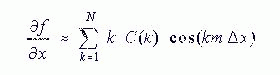
3. Derivatives are by summing derivatives of each basis function:
|
|||||||||
|
4. Increase the resolution by choosing a smaller grid point interval:
i.e. smaller dx. This means more grid points
at which to make calculations.
|
4. Increase the resolution by choosing a larger maximum wavenumber k.
(Larger k is a smaller wavelength.)
|
|||||||||
5. Advantages:
|
5. Advantages:
|
|||||||||
6. Disadvantages:
| ||||||||||
|
| ||||||||||
|
| ||||||||||